Machine Learning Resources:
To many of those within the biological sciences that lack a computational or mathematical background, “machine learning” exists as a confusing and daunting topic. While some of the specific concepts in machine learning can certainly be complex and involved, on a practical level, the underlying principles of machine learning are rather intuitive and approachable. One of the motivating forces behind PARROT is to bridge this divide between complexity and accessibility. With PARROT, our lab aims to provide users with a robust machine learning framework that is easily-useable, even for those with little-to-no exposure to machine learning.
This document provides a high-level background on some of the pertinent machine learning concepts present in PARROT. Additionally, I hope to point out common pitfalls to avoid when using PARROT, or any other machine learning tool. Wherever possible, relevant papers, articles, and blog posts will be linked in order to provide a more thorough description of these concepts.
First things first, what is ‘Machine Learning’?
Broadly speaking, machine learning describes a class of computer algorithms that improve automatically through experience. While the idea of machine learning has been around for over 50 years, modern advances in computing hardware and machine learning algorithms, along with the universal growth of ‘big data’, has caused the field to gain widespread popularity. Today, ML has been adopted by a whole host of applications, ranging from computer vision, language processing, advertising, banking and many many more. In particular, ML is becoming increasingly common within the biological research community in coordination with the massive increase of raw data from high throughput sequencing, proteomics, metabolomics, and other data generating techniques. Although their effectiveness is not unlimited, ML approaches are capable of identifying patterns in data that would otherwise go unnoticed.
Helpful resources:
When can I use machine learning for my research?
Machine learning approaches like PARROT are great for data exploration and hypothesis generation. When facing a large set of biological data, ML can help you identify patterns in your data and allow you to design testable predictions based on those patterns. However, it is important to note that ML generally cannot validate a result on its own, and is most effective when combined with follow-up experimental validation.
There are two primary types of problems that machine learning is designed to address: classification and regression. As the name implies, classification is the process of assigning new datapoints to particular, discrete classes. For protein data, questions involving things like cellular localization, presence of PTMs, presence of a molecular interaction, etc., can be framed as classification problems. In contrast, regression problems involve assigning each data point a continuous real number value. For example, proteins can be assigned values corresponding to their expression levels, disorder, binding affinities, etc.
Helpful resources:
What is a recurrent neural network (RNN)?
A recurrent neural network is a particular machine learning framework specifically designed for answering questions involving sequential data. RNNs were originally designed for tasks in the field of language processing (since language is essentially just a sequence of words), but in recent years they have been applied more broadly in the biological sciences. In particular, RNNs have seen promising use in analyzing protein sequences.
Part of the rationale for using RNNs for PARROT is that they are capable of taking in variable length sequences as input. Traditional neural network architectures require a fixed-length input, so for this proteins have to be split into fixed-sized fragments by running a sliding window across the entire sequence. From a practical standpoint, this kind of approach can be quite effective. However, it introduces extra hyperparameters (window size and stride length) that need to be tuned, and is not always optimal for identifying longer-range effects. In contrast, RNNs do not require sequences to be split or padded before being run through the network. More details on the architecture of RNNs can be found at the links below.
There are a few variations of RNN architecture that PARROT utilizes to achieve optimal performance. The first is the bidirectional recurrent neural network, or BRNN. Standard RNNs process sequence information one input at a time in the forward direction. So for protein sequences, this would mean looking at the sequence on amino acid at a time from the N-terminus to the C-terminus. BRNNs build on this architecture by also having neural network layers that process information in the reverse direction, then aggregate the information from the forward and reverse layers. PARROT implements a BRNN because the convention of writing proteins N-to-C is relatively arbitrary, and a bidirectional approach enables the network to capture more relevant information from the primary sequence. The second variation on RNNs used by PARROT is a Long Short Term Memory (LSTM) architecture. LSTMs fix some of the issues present in standard RNNs and improve the network’s ability to learn long-range effects present in the data.
Helpful resources:
What are the hyperparameters of the networks used by PARROT? What should I set them as?
‘Hyperparameters’ in machine learning are parameters governing the architecture or learning ability of a neural network that can be tuned to impact overall performance. The networks used in PARROT have a few hyperparameters that the user can specify, or can be optimized automatically. These hyperparameters are:
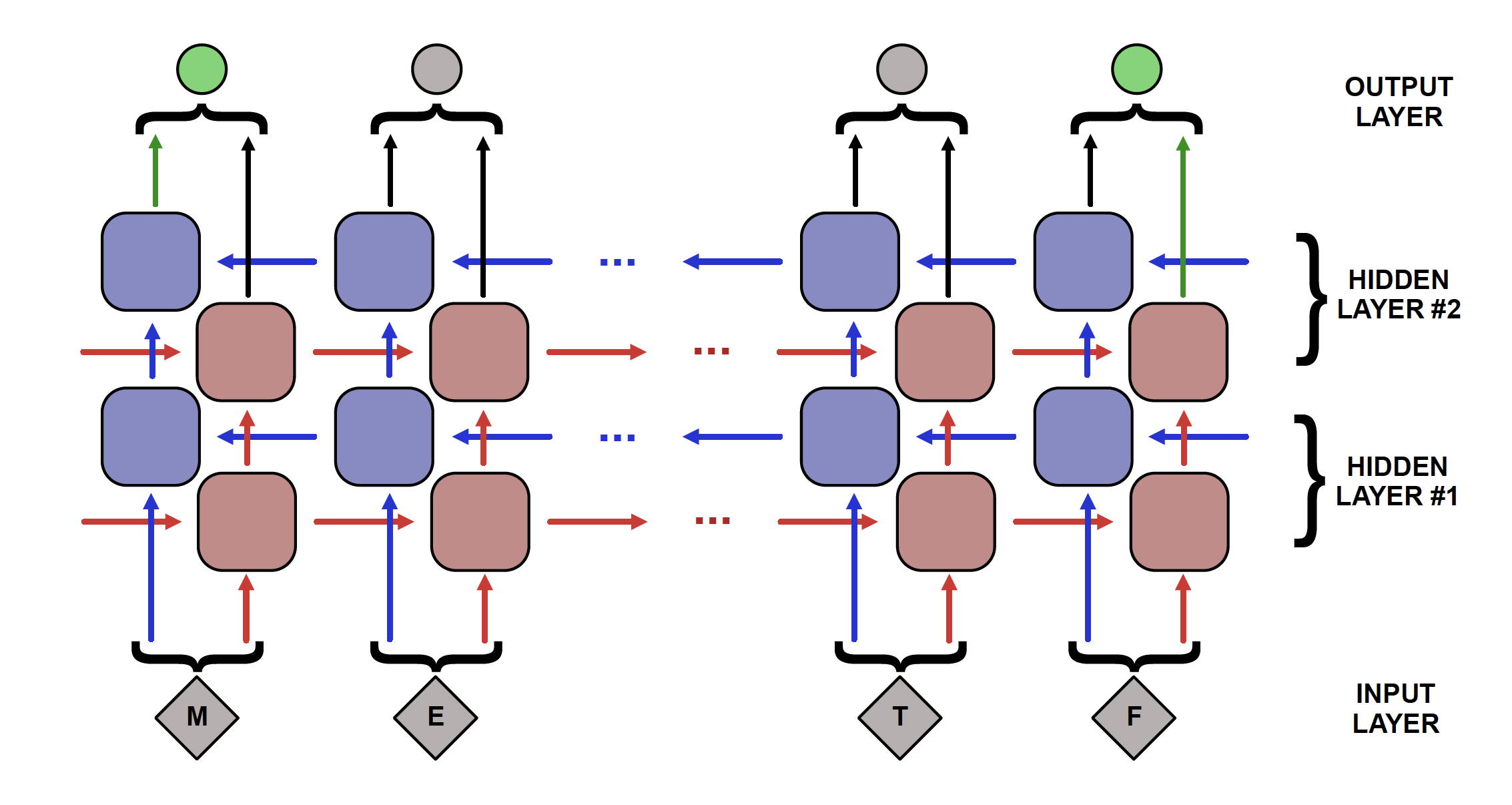
Number of hidden layers (’–num-layers’ / ‘-nl’): In a recurrent neural network, each layer constitutes a set of nodes to propogate information from one end of the sequence to the other. The most simple kind of RNN has only a single layer that processes input and produces output. However, an RNN can consist of multiple layers of sequence-spanning nodes. In this case, the first layer still processes input as before, except now this layer’s output is passed as input for the next layer. For bidirectional RNNs, each layer specified by this parameter consists of both a forward and backwards layer, so specifying ‘–num-layers 2’ will create a network with 2 forward and 2 backwards layers.
An RNN with many hidden layers is said to be “deep”. In general, a deeper network is capable of identifying more complex patterns since there are more degrees of freedom within the network. However a deeper network also has the drawbacks of taking significantly longer to train and having a greater likelihood of overfitting the training data. Choosing the optimal depth of a network is highly dataset-dependent and a non-trivial problem in the field of machine learning. Ideally, a network will be as simple (“shallow”) as possible while also performing well on the task at hand. In practice, networks with 1-4 layers tend to perform well on most tasks and improvements for using deeper networks is small, but PARROT provides the user with the option. PARROT also has a built-in optimization procedure for determining the depth of the network given the data, which can be useful for extended analyses of a dataset.
Hidden vector size (’–hidden-size’ / ‘-hs’): A hidden vector in an RNN refers to the “packet” of information that is transmitted from one node to the next. If the hidden vector has a size of one, then only a single number is transmitted, if it has a size of 5 then 5 numbers are transmitted. Vectors of this size pass information both “laterally” across a layer as well as to the next deeper layer in the network.
The pros and cons of using a larger hidden vector size are similar to the number of layers hyperparameter, though the effects are less dramatic. Using larger vectors can be useful for more complex tasks, at the expense of computational speed and overfitting. As with number of layers, hidden vector size is also a hyperparameter that can be optimized for a dataset by PARROT.
Learning rate (’–learning-rate’ / ‘-lr’): In machine learning, learning rate is a proportionality constant between 0 and 1 that affects the extent to which the weights in the network are updated after every round of training. A learning rate of 1 would cause very large updates of the weights, and a learning rate of 0 would cause the weights to remain constant throughout training. Large learning rates also tend to cause the network to train more quickly. A typical learning rate for machine learning is either 0.001 or 0.0001 as these tend to produce steady and gradual learning, though the optimal learning rate for a task is dataset-dependent. If the learning rate is too large, the network weights will experience large fluctuations and may not find the optimal values. In contrast, if the learning rate is too low, the network weights can get stuck in local minima and fail to find the optimal values. In practice, many machine learning applications rely upon algorithms called optimizers (PARROT uses the Adam optimizer) that adjust learning rate over the course of training in order to achieve optimal network performance. So for PARROT, the user-specified ‘–learning-rate’ hyperparameter sets the initial learning rate, though this can also be automatically selected by running parrot-optimize.
Batch size (’–batch’ / ‘-b’): Although most depictions of machine learning show a network processing one piece of data at a time, this is not very computationally efficient nor is it the most effective way of training a network. Rather, data is often grouped together into “batches” that are run through the network simulataneously. It is faster for computers to process data in these larger groups, especially when the computer has GPUs available for training. Running data together in batches also leads to more “averaging out” of errors during training, which can make training occur more smoothly.
Selecting the right batch size largely depends on the overall size of the dataset. It’s not typically recommended to use a batch size larger than 256. Typically, a batch size that is around 1-10% of your overall dataset works well. Batch sizes slightly smaller or larger than this do not really effect overall performance, so it is not the most crucial hyperparameter to tune. A good default value for batch size is 32.
Number of epochs (’–epochs’ / ‘-e’): In machine learning, an epoch is a round of training. Each epoch the network will “see” each item in the training set once. As one might expect, a larger number of epochs means that the network will train for longer and will lead to better performance up to a point. Too many training epochs will eventually cause the network to overfit on the training data, which will hurt network performance on non-training data. However, PARROT has features implemented that prevent this kind overfitting, so specifying a large number of training epochs should not hurt overall performance. For more details, read the over- and under-fitting section below.
Helpful resources:
What is ‘encoding’?
Encoding is the process of converting input data into a format that neural networks can read. For PARROT, that means converting protein sequences into a numerical representation. There are several possible ways that a protein sequence can be encoded. The most basic is one-hot encoding, the default for PARROT, which represents each amino acid as a length 20 vector, where 19 positions contain the value ‘0’, and 1 position contains ‘1’ depending on the identity of the amino acid. Other encoding schemes aim to represent more similar amino acids, like Glu and Asp, as having more similar encoding vectors than other unrelated amino acids. For example, one can encode each amino acid on the basis of their biophysical properties like charge, molecular weight, hydrophobicity, etc. While naturally one might assume that this kind of biologically relevant encoding scheme would be more effective for machine learning tasks, that is actually not the case. The paper referenced below showed that for many tasks, one-hot encoding actually performs as good as or better than biophysical scale encoding. The reasons for this are not entirely clear, but it illustrates the potent ability of ML to identify patterns in data.
Helpful resources:
What are over-fitting and under-fitting?
Even when working with a large dataset, your dataset will never be completely representative of the entire space of possible data. The whole purpose of machine learning is to learn patterns from your labeled dataset (i.e. data where the underlying values are known) and extend it onto new, unlabeled data (where the underlying values are not known). As one might imagine, the ability of a machine learning network to extract these patterns heavily depends on the characteristics of this labeled data. One of the most common issues encountered in machine learning is over-fitting, which is when your network is trained such that it can perform well on the dataset it learned from, but its performance is not generalizable to outside data. Over-fitting can be the result of overtraining, or due to how the dataset is structured. The following section describes in more detail how one should go about setting up their dataset to avoid overfitting, and here I will briefly describe the techniques that PARROT employs to prevent overtraining.
As ML networks train on a dataset, they become better and better at predicting the data they are seeing. For a sufficiently complex network, after infinite training epochs the network will achieve 100% accuracy on the training dataset. However, for practical purposes this is not particularly helpful, since the “ground truth” of the training dataset is already known. Rather, we are interested in the performance of the network on unseen data. Many machine learninig approaches, including PARROT, approximate this unseen data by partitioning and setting aside a small chunk (often 10-20%) of the data and designating this as the validation set. This set of data is not used at all for the actual training of the network. Instead, after every epoch, the performance of the network on the validation set is evaluated. If training for an infinite number of epochs, the performance on the training set (AKA “training loss”) will continue to improve, but after a while the performance of the validation set (AKA “validation loss”) will plateau, then eventually decline as the network begins to overfit the training set. The state of the network when the max validation set performance is achieved is ultimately what is conserved after training.
In PARROT along with other ML applications, this partitioning of the data is actually taken a step further as well. The original data is actually divided into three groups: the training set (~70%), the validation set (~15%), and the test set (~15%). Training procedes as described in the previous paragraph. After training, the network is evaluated one final time on the test set, which it has never seen up to this point. The purpose of this step is because since the the test set is totally unseen, it can provide a good estimate of how well the final network will perform on new, unlabeled data.
So far I have described over-fitting, but under-fitting can also be a problem in machine learning. Underfitting occurs when your network is not complex enough to capture the patterns in the data. The mathematical representation of this would be trying to fit a line to a set of points generated from a parabola–it doesn’t matter how long you train, there is just a finite limit of how accurate your model will be. The solution to underfitting is to use a more complex machine learning model. For PARROT this would entail specifying a larger number of layers or larger hidden vectors within the network.
Helpful resources:
How should I set up my dataset?
Even with all of the bells and whistles associated with modern neural network architectures, by far the most important step in any ML pipeline is the initial data processing. As such, this should be carried out diligently, with checks along the way to make sure everything is in order. Errors in your dataset can result in networks that fail to learn the patterns in the data entirely, or more insidiously, networks that appear to learn, when in reality they are not. Ultimately, being careful when setting up your dataset can save a lot of time troubleshooting down the road.
There are two important considerations in ML regarding your data:
Make sure you have balanced classes or an even distribution of regression values. What this means is that if you are addressing a classification task, each of the classes should have a roughly even number of datapoints in your dataset. For example, if you have three classes in a 1000-item dataset, ideally each class would compose ~300-400 of those datapoints. Likewise, for regression tasks, ideally your datapoints will have a roughly uniform distribution across the range of regression values. The reason why a balanced dataset is important is because inbalanced data will bias your network towards predicting the over-represented class. To illustrate this point, take the following case:
You are working with a dataset in which you have 1000 labeled protein sequences that all belong to either ‘Class A’ or ‘Class B’, as well as another group of proteins for which you would like to predict what class they belong to using ML. In the extreme case, if every sequence in your dataset belong to Class A, then your ML approach will “learn” that every single sequence should be assigned Class A. After all, the strategy of “predict everything as A” has worked well for your network during training, so this will not be a very generalizable predictor. Even if the dataset is skewed 80%-20% in favor of Class A, the network is likely to predict Class A when facing any uncertainty, since statistically this is a good strategy to minimize loss.
By default, PARROT will output warnings in cases where a dataset is obviously imbalance (both for classification and regression).
Limit similarity between samples in your dataset. The issue with having similar samples arises when the similar samples are split between the training set and the validation set or test set. If this happens, your network will have artificially inflated performance and a tendency to overfit your data.
For example, imagine you have a protein dataset where half of the proteins come from the human proteome and the other half are orthologous proteins from the mouse proteome. If the network is trained on human protein A, if it encounters mouse protein A in the validation set, it will probably have an accurate prediction since these proteins (in most cases) will have highly similar sequences and will be functional orthologs. Thus the network will be incentivized to overfit the training data, rather than develop a generalizable predictive model. Likewise, if the data is split such that human protein B is in the training set and mouse protein B is in the test set, the network will perform better on the test data and give an inflated view of how accurate the network truly is on unseen data.
Fortunately, this problem is fairly easy to correct for with protein data by removing samples that display similarity above a certain threshold. If for some reason highly similar sequences can’t be removed, then care should be taken so that similar sequences are grouped together in the training set, validation set, or test set. As a basic check, PARROT will warn users if there are duplicate sequences in their dataset.
Helpful resources:
How should I tackle a huge dataset?
Although larger datasets tend to yield more accurate ML networks, it also makes training a network much more time consuming. With PARROT, trying to optimize hyperparameters an a large dataset can take an unreasonably long time. There are a few possible ways to speed up this process.
Train on a computer with GPUs. PARROT is optimized to train in parallel on machines with GPUs, so if available, this can speed up training up to 10- or 20-fold.
Optimize hyperparameters on smaller, representative subset of the data. Although ideally you would optimize hyperparameters on the entirety of the data, this is not feasible on sufficiently large dataset. Instead, you extract a subset of the data (still considering the points about dataset structure from the preceding section) on which you can tune the hyperparameters. Once the best hyperparameters are determined, you can train on the entire network.
How can I validate that my trained network is performing well?
Since machine learning approaches tend to function as “black boxes” that cryptically make predictions given a set of input data, a critical challenge for users is being able to validate that their network is making generalizeable and accurate predictions. In general, there are two ways one can validate their trained networks:
Validate on external, independent data
This is the best-case scenario. In an ideal world, you should evaluate your network on data that was collected in a manner completely independent from the dataset you used to train the network, either via different techniques or different underlying sources. By comparing the predictions made by a network to this independent “ground truth”, you can ensure that your network is not overfitting to particular features/biases inherent in your training dataset.
Intra-dataset validation using cross-validation
Unfortunately, in many cases there aren’t any independent datasets that you can use to validate your network! The solution developed by the machine learning community in these cases is to approximate an independent dataset by “holding-out” a subset of your data during training and evaluating how your network performs on this data. As described above, PARROT employs this sort of a test set by default, and even produces an output “_predictions.tsv” file that compare the test set predictions to the true scores. Careful analysis of this file can reveal potential biases in your network.
Extending this idea of a held-out test set, a commonly-used practice called cross-validation enables using an entire dataset as test data for validation. The first step of the cross-validation procedure entails dividing a dataset into K (typically K=5 or K=10) even sized chunks (termed “folds”). The network is then trained K different times, with a different fold being used as the test set in each iteration while the remainder are used to train the network. At the end, the predictions for each test set (i.e., the full dataset) are combined or averaged to produce a more robust estimate of network performance. Finally, the entire undivided dataset can be used to train a final network which should have similar (or better) performance than what is estimated by the combined cross-validation test sets.
PARROT includes several tools which facilitate cross-validation training, and a comprehensive example is provided on the “Evaluating a Network with Cross-Validation” page.
NOTE: Cross-validation is also often used to select the best hyperparameters for machine learning networks (it’s used by parrot-optimize). This is a nearly identical procedure to what’s described above, but hyperparameter tuning and network validation are NOT the same thing. Estimates produced by hyperparameter tuning can be overly optimistic compared to how your network would actually perform on data it’s never encountered before.
Helpful resources:
What are the different performance metrics for evaluating ML networks?
PARROT outputs a number of figures and performance stats to let user’s know how accurate their trained networks are on held-out test data. These performance metrics can be useful snapshots for comparing different network architectures and training strategies, and as a result, many are widely used within the field of ML. While our intention in designing PARROT was to make this output information convienent and helpful, users should still carry our more comprehensive analysis directly on the predictions file (“_predictions.tsv”).
The performance metrics used for assessing classification performance and regression performance are quite different. In classification tasks, it’s common to make a confusion matrix for comparing predictions to ground truth class labels. The classification metrics used in PARROT are all derived from these matrices.
The most simple of these metrics is Accuracy, which simply denotes the fraction of correctly classified samples. Accuracy is practical and easy-to-understand, but is not as useful of a metric for imbalanced datasets. For example, if your dataset is 80% Class A and 20% Class B, a network that predicts all samples to be Class A would have an accuracy of 80%, even though it completely fails to discriminate between classes. This sort of network is obviously less useful than a different network that is 80% accurate, but with a more even distribution of incorrect classifications. F1 score and Matthews Correlation Coefficient (MCC) are two metrics that take into account the balance between false positives and false negatives. F1 score is more widely used, but MCC is generally viewed as a more comprehensive metric (see link below). Like accuracy, the ideal MCC and F1 score are ‘1’. Together these three metrics effectively describe how well a classifier is performing.
Training a PARROT network in probabilistic-classification mode will also produce a Receiver Operating Characteristic (ROC) curve and a Precision-Recall curve, with their corresponding areas. For these metrics, an area under the curve of ‘1’ denotes a perfect predictor. These curves are generated by varying the prediction threshold and seeing how the relative false positive and true positive rates vary (ROC) or how precision and recall vary at these different prediction thresholds. ROC curves are more common, but for imbalanced datasets, area under the PR curve is a more useful metric.
The standard way of evaluating regression networks is to make a scatterplot comparing the correlation of predictions to ground truth values. Two ways of measuring correlation are with Pearsons correlation and Spearmans correlation. These metrics are similar, but have a few subtle differences. Pearsons correlation, or Pearsons R, directly measures linear correlation (i.e., how well does a line fit the data). Spearmans correlation measures rank order correlation. As a nonparametric method, Spearmans correlation can detect correlations that are monotonic, but nonlinear. Spearmans correlation is more robust to outliers, and does not make assumptions that the underlying data is normally or uniformly distributed. Like the classificaiton metrics, these two metrics are quite similar in most realistic cases.
Helpful resources:
How does PARROT choose the optimal hyperparameters?
As described above, there are several different RNN hyperparameters that affect network architecture and training. In general, there is not hard and fast rule for selecting what these hyperparameters should be set at, since it varies from dataset to dataset. Since using different hyperparameters can have a noticeable impact on performance, people have developed algorithms for selecting the optimal hyperparameters for a given dataset. All of these algorithms take the general form of: 1. iteratively select hyperparameters by some criteria; 2. train a network on the data using these hyperparameters; 3. evaluate the performance of this network; and 4. pick the hyperparameters that yielded the best-performing network.
The most simple optimization algorithms are grid search and random search. These are iterative approaches that sample many points in hyperparameter space either systematically or randomly, respectively. As you can imagine, searching many combinations of hyperparameters is likely to find the best-performing set. Unfortunately, these approaches can be very time consuming and are not often used for more complex machine learning problems.
Instead, PARROT implements a technique called Bayesian Optimization to select the optimal hyperparameters for a given dataset. The details of this method are more involved than I will describe here, but below are several resources that do a good job explaining the algorithm. Briefly, instead of performing an iterative search over the hyperparameter search-space, Bayesian Optimization relies upon the mathematical concept of a Gaussian process (GP). GPs can estimate the loss function across all of hyperparameter search-space. Initially, this estimate is not very accurate, but as you train and test more sets of hyperparameters, the estimate becomes more accurate. The upshot is that Bayesian Optimization can generally identify the optimal hyperparameters in much fewer iterations than grid or random search.
Helpful resources: